Data Visualization
Goal
How to visualize data using R package ggplot2.
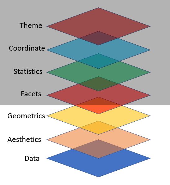
ggplot2 Layers
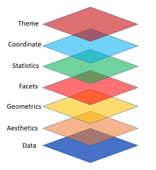
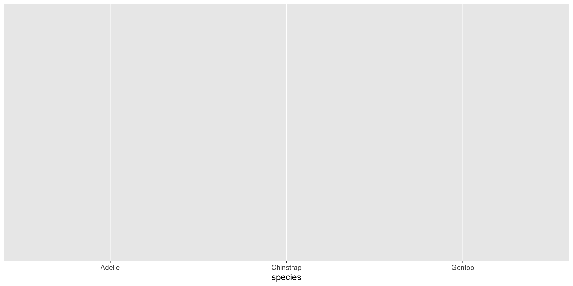
Import Data

Map Variables Aesthetics
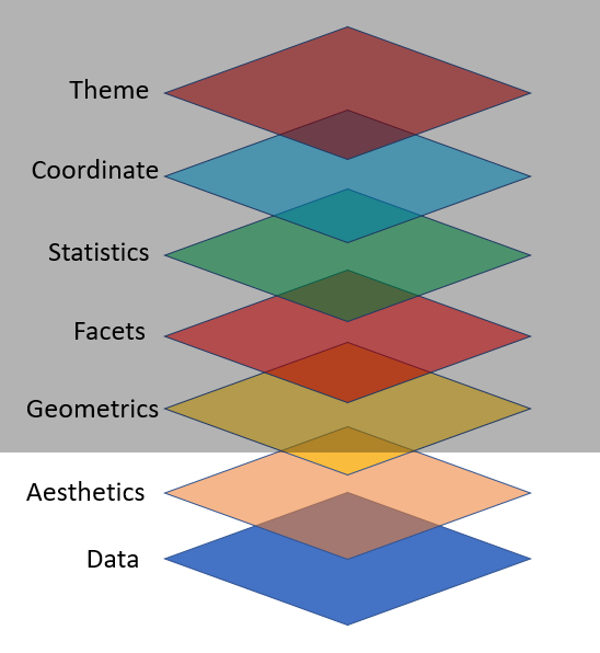
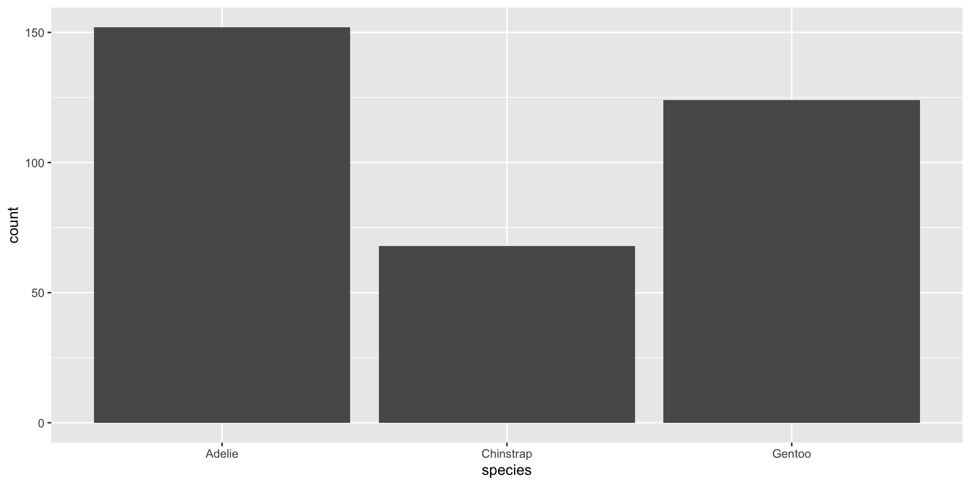
Add Geometric Shapes
🧠 YOUR TURN
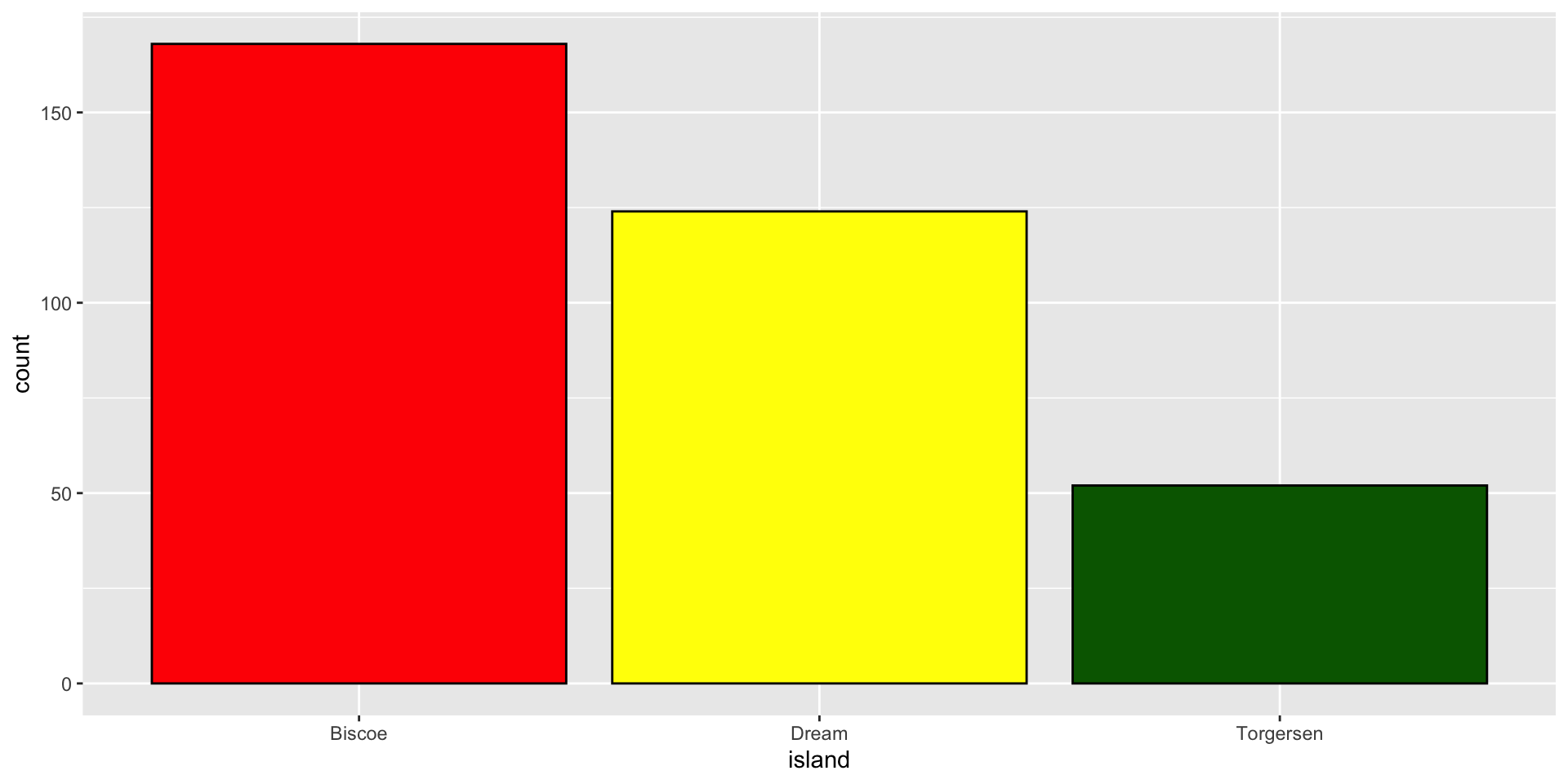
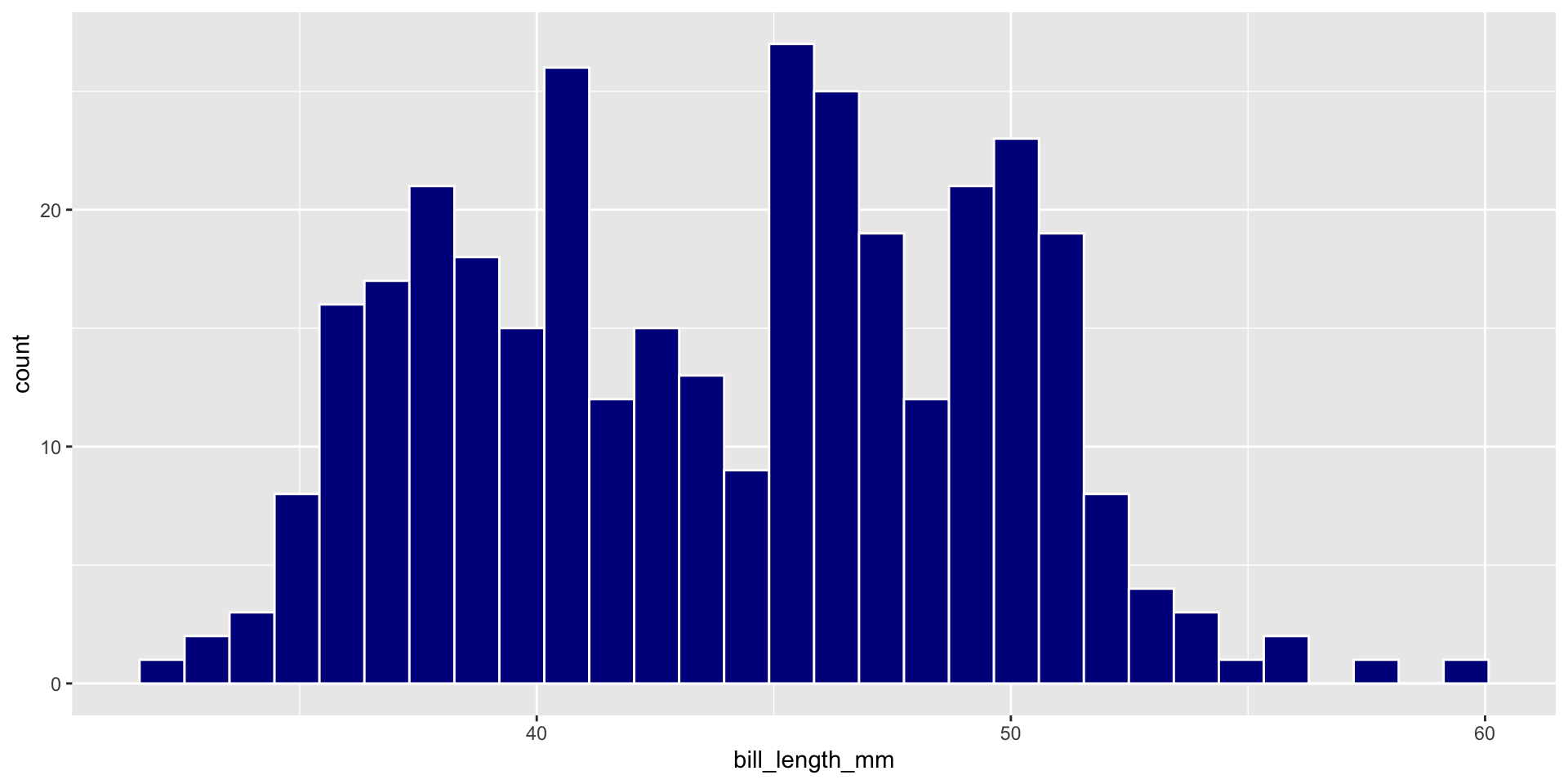
“Fill” Color
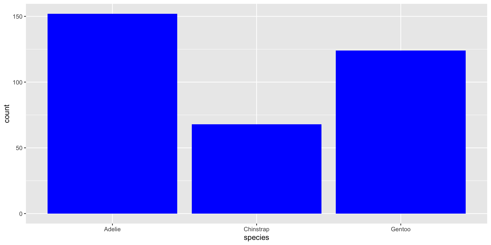
“Fill” Colors
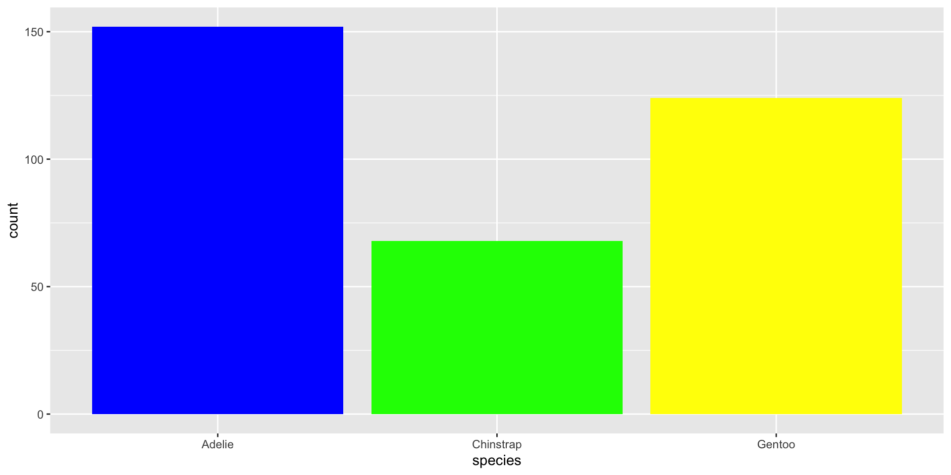
“Fill” & “Color” Colors
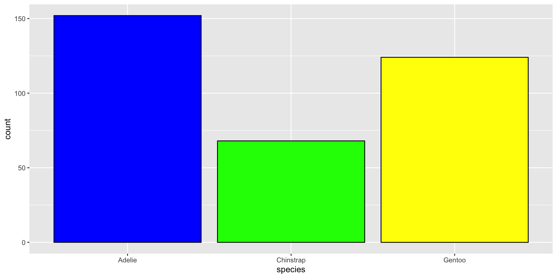
🧠 YOUR TURN
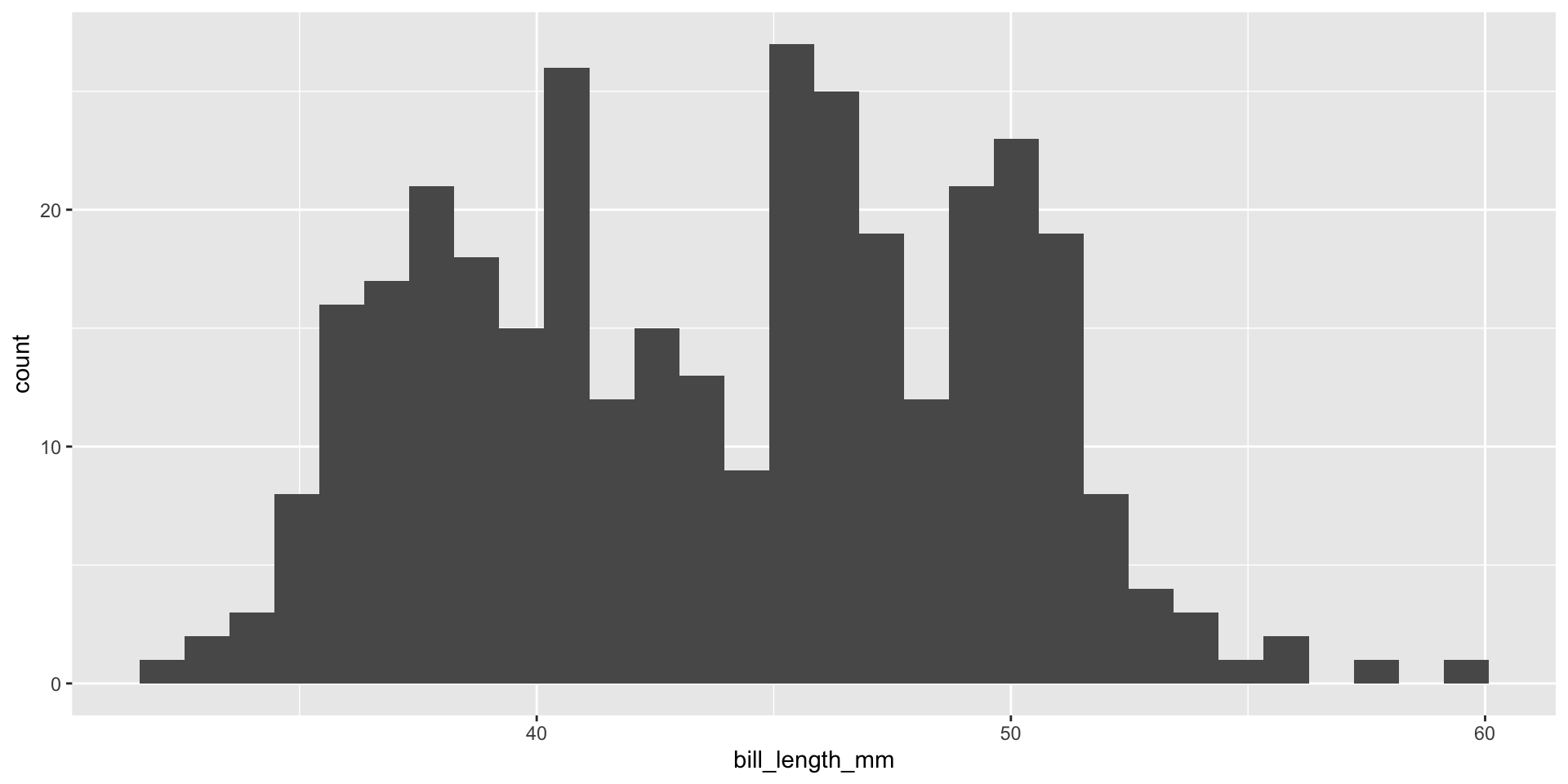
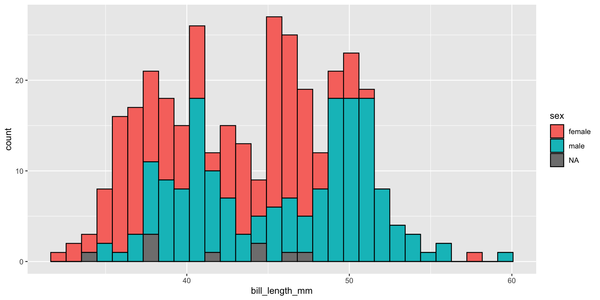
Plot A Continuous Variable
🧠 YOUR TURN
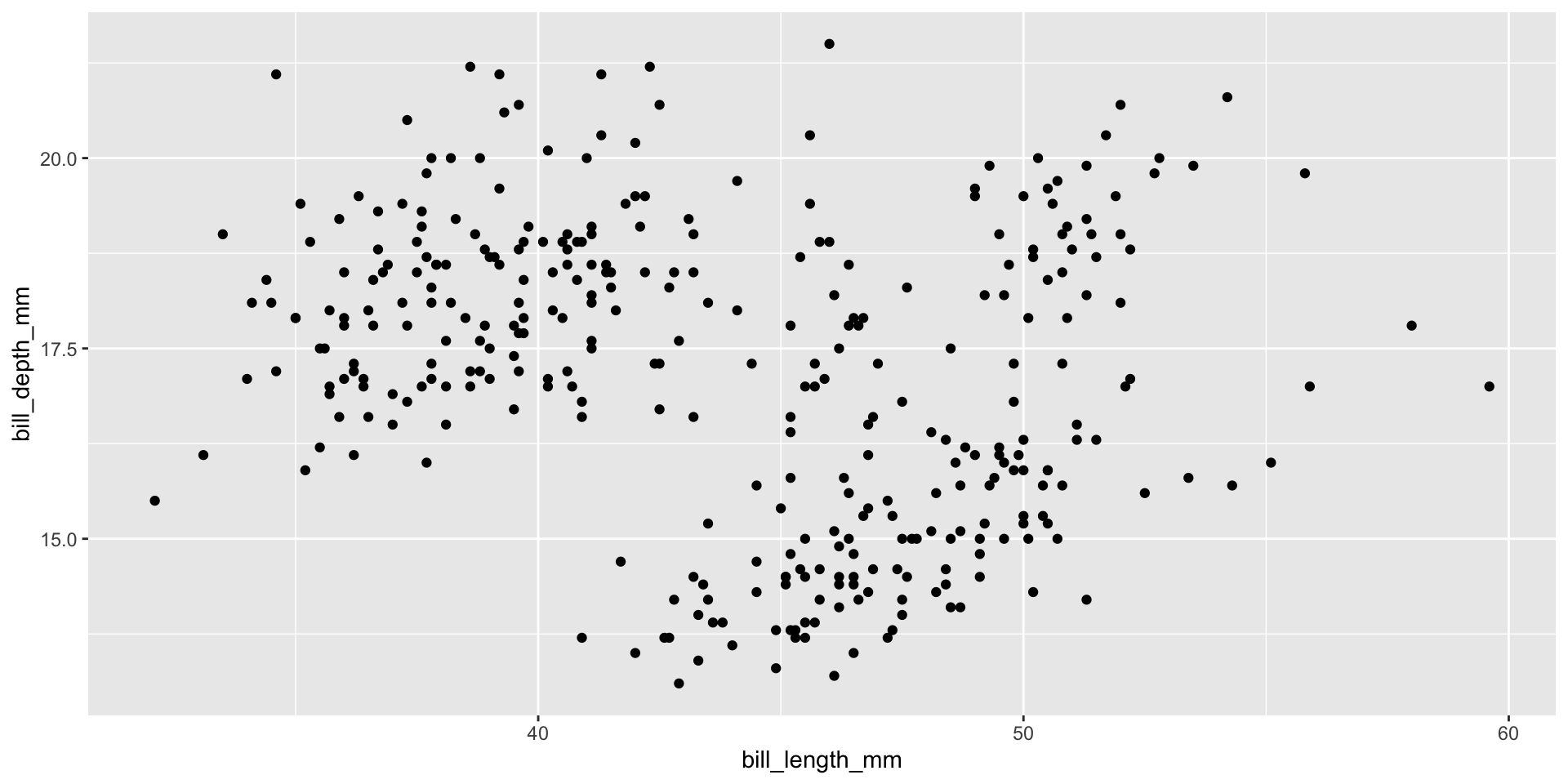
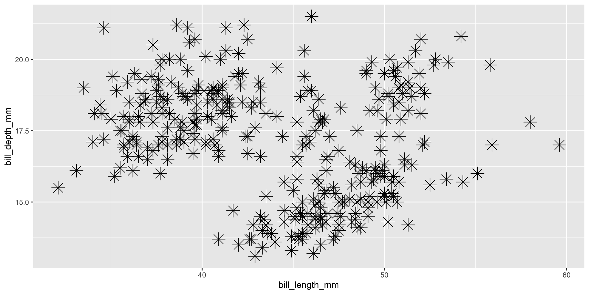
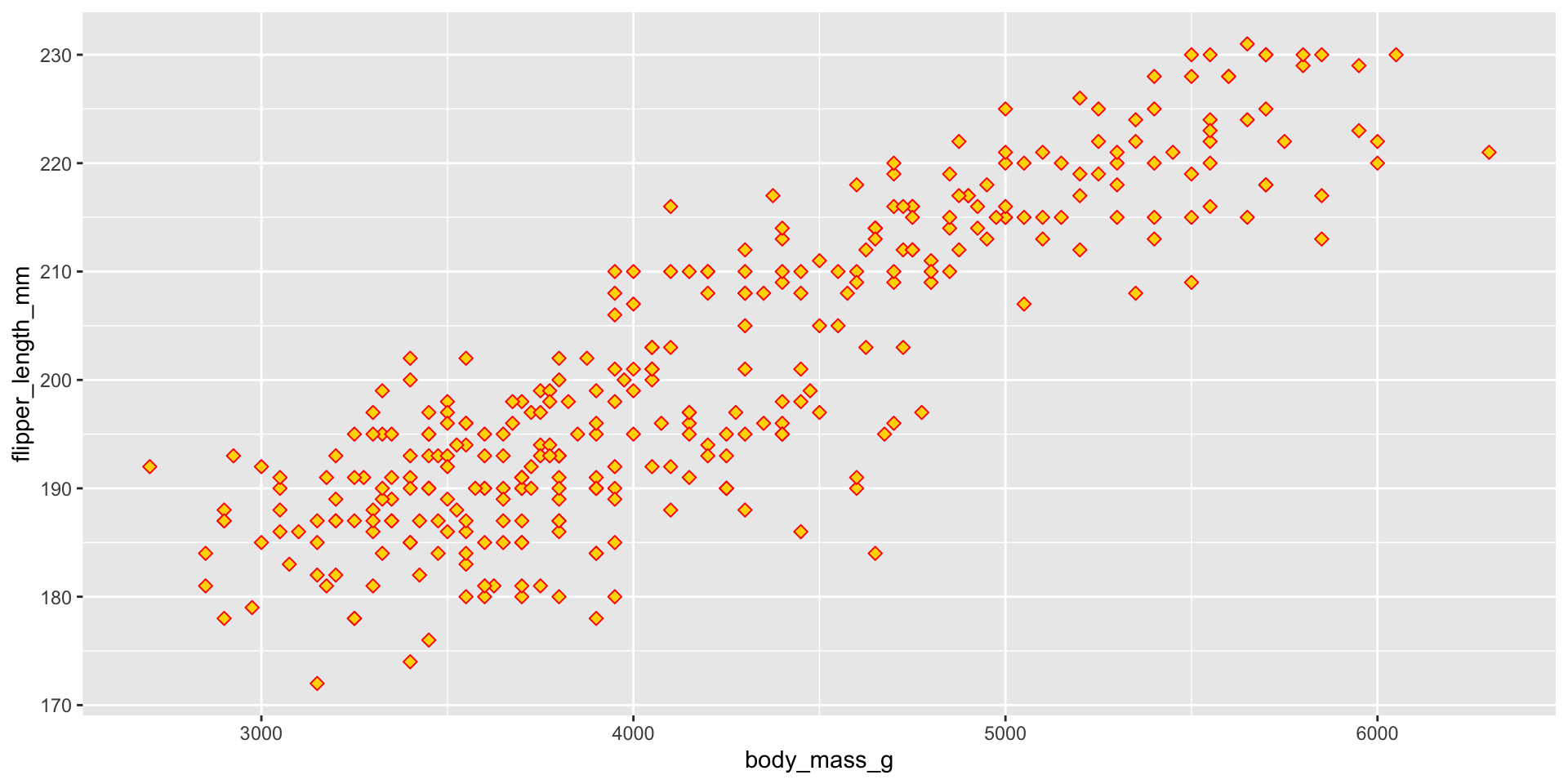
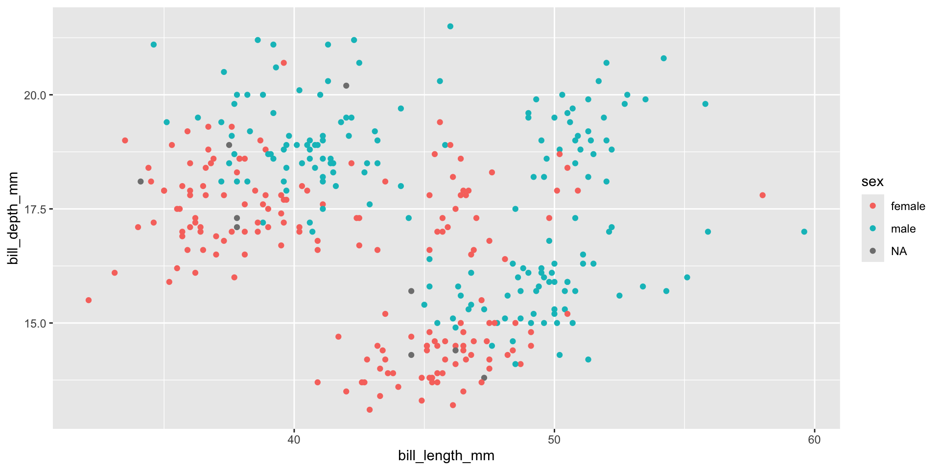
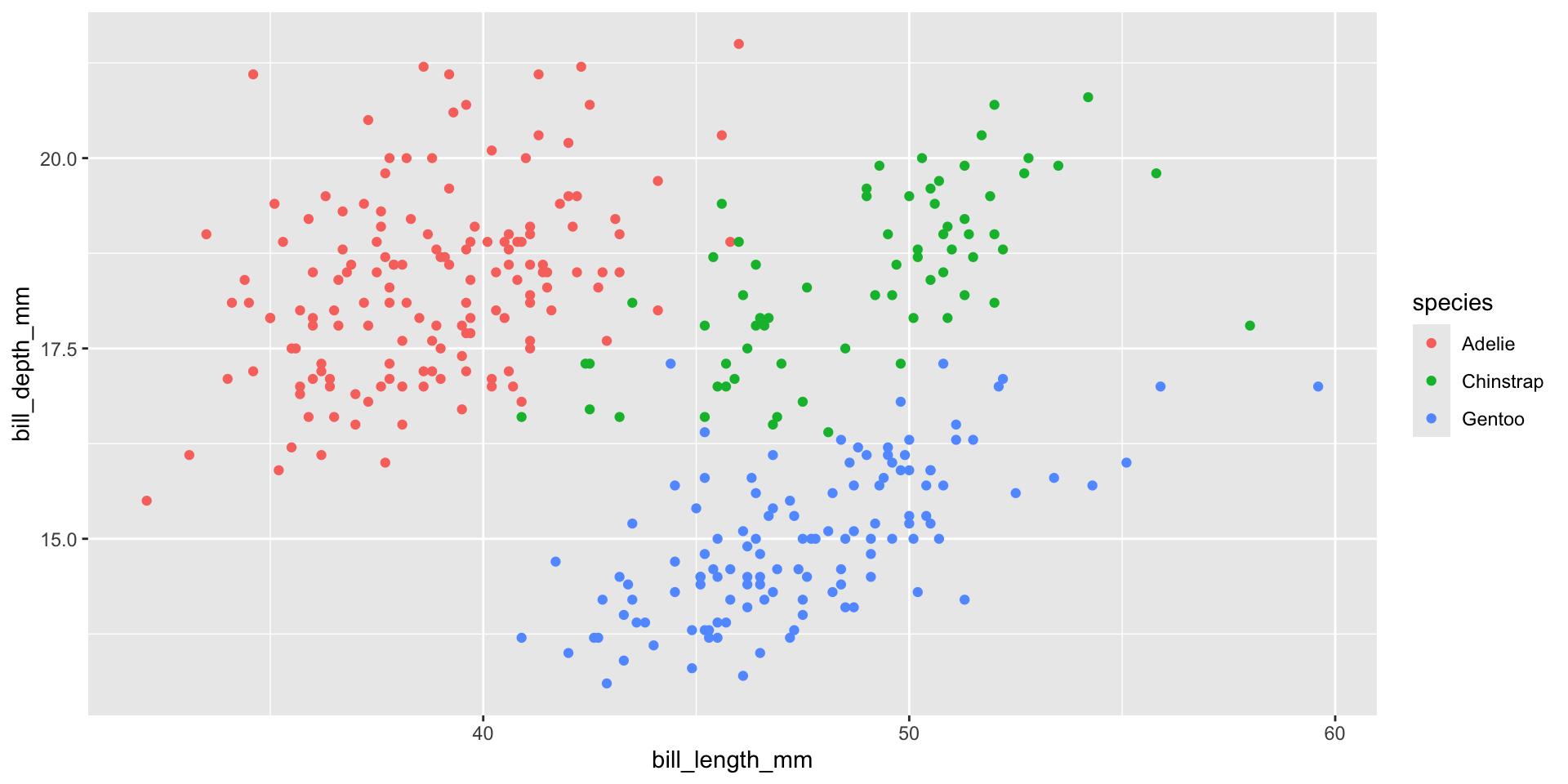
Two Continuous Variables
Geom Size
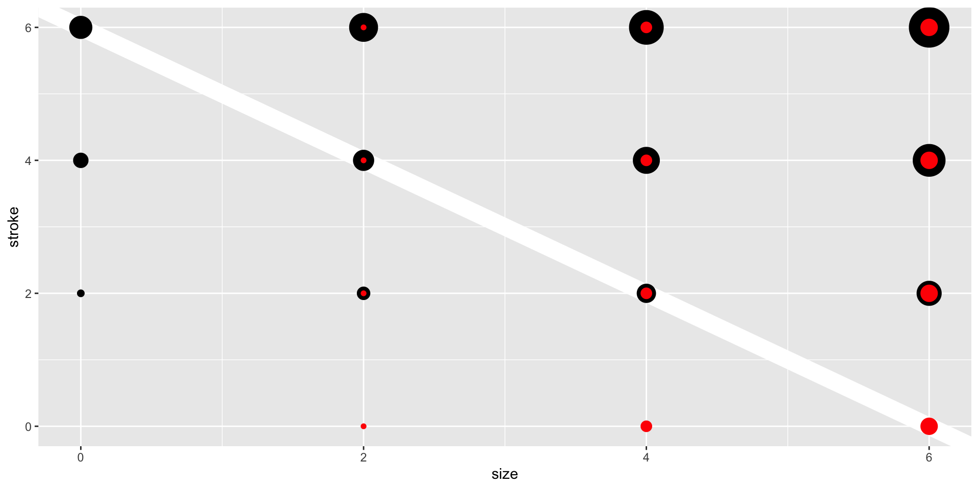

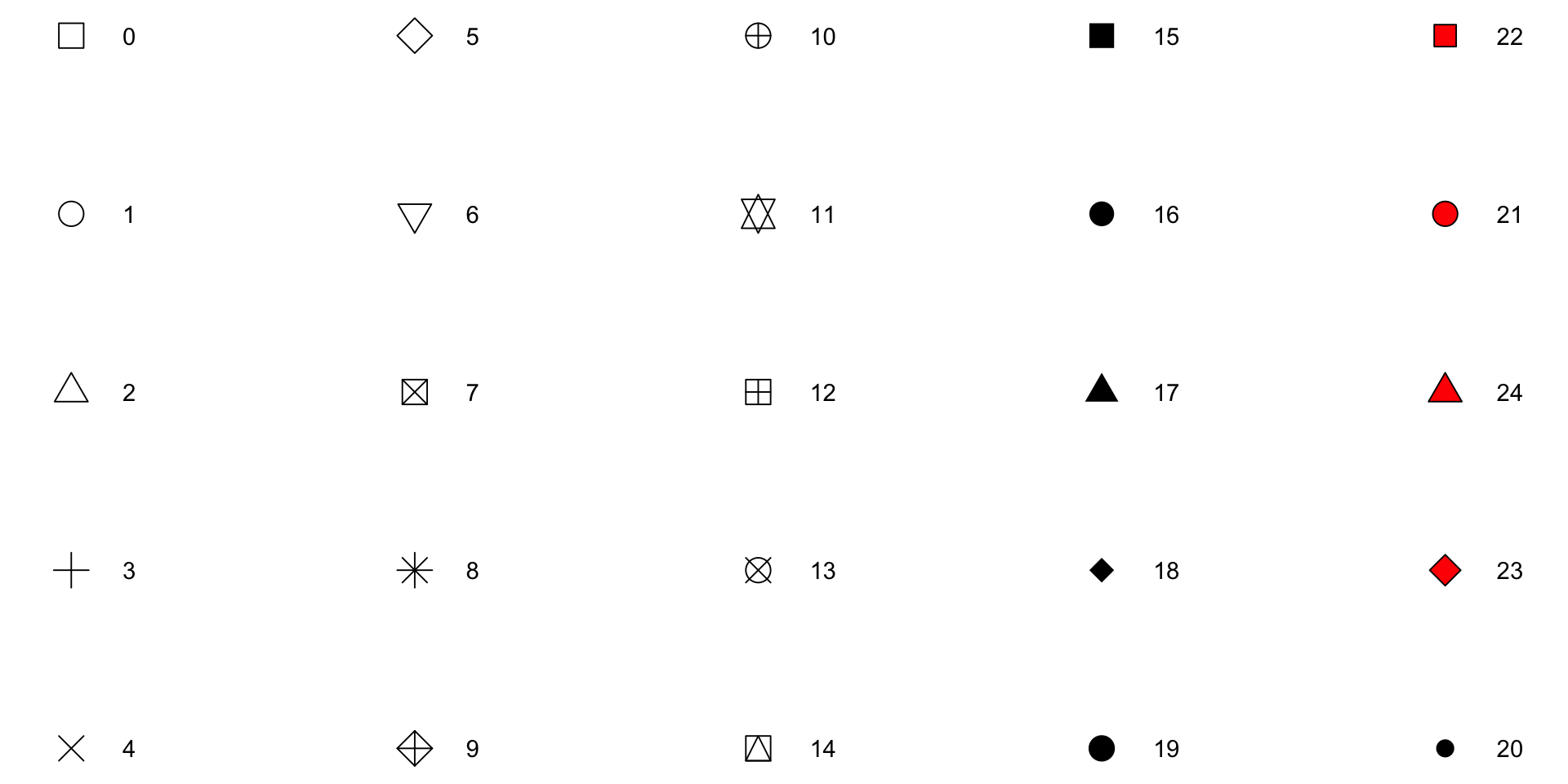
Geom Shape
🧠 YOUR TURN
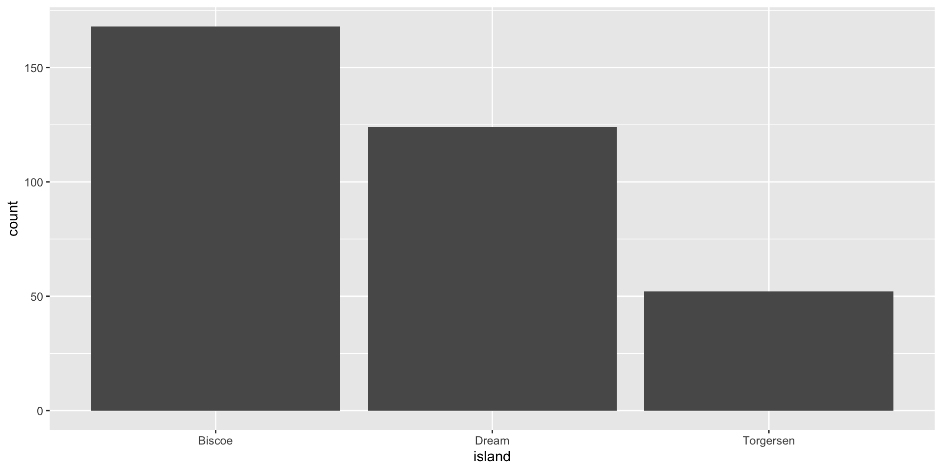
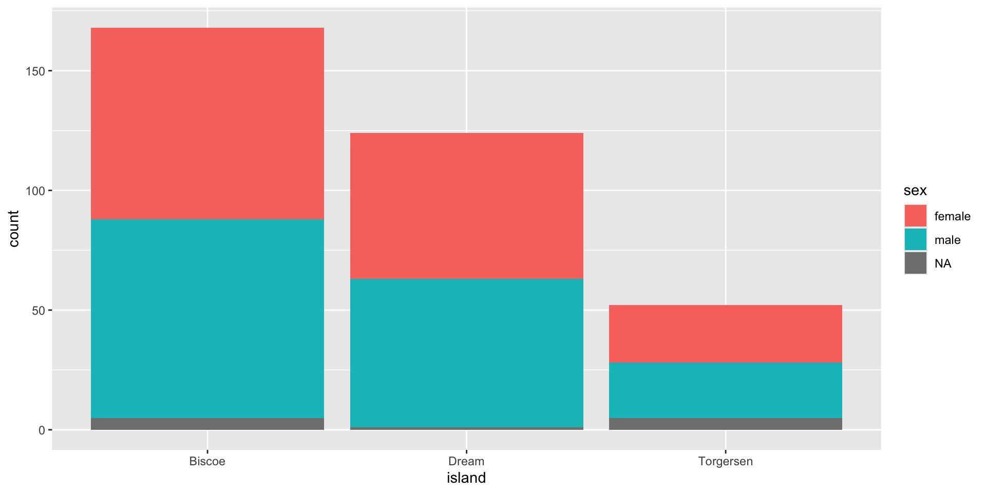
Plot A Factor & Factor
Plot A Factor & Continuous
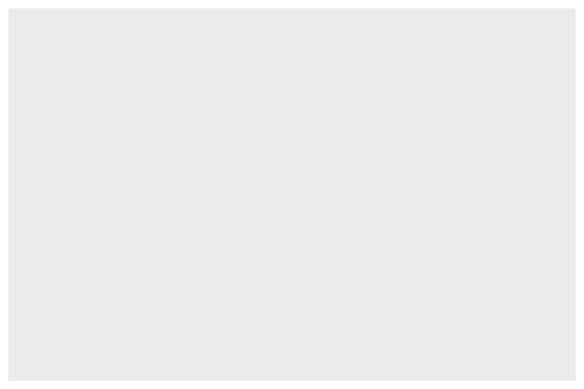
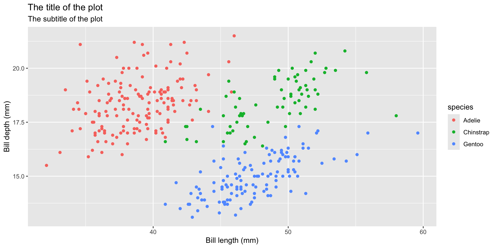
A Factor & Two Cont.
A Factor & Two Cont.
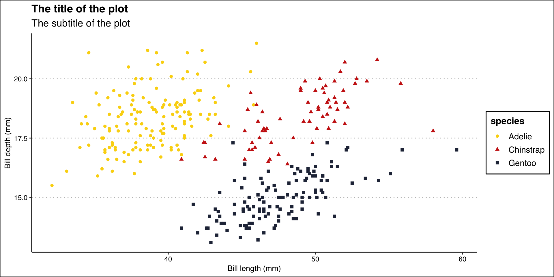
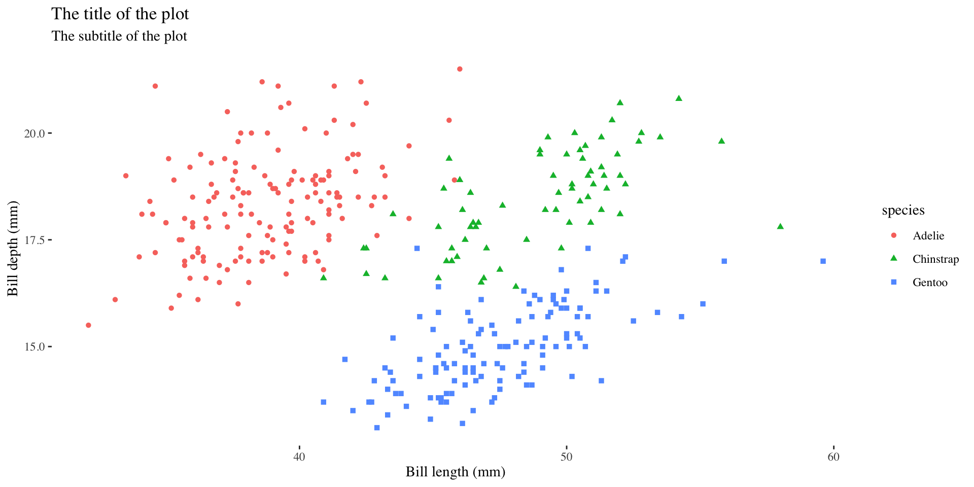
Write Labels
Title of the plot
Subtitle of the plot with more information
Title of the x-axis
Title of the y-axis
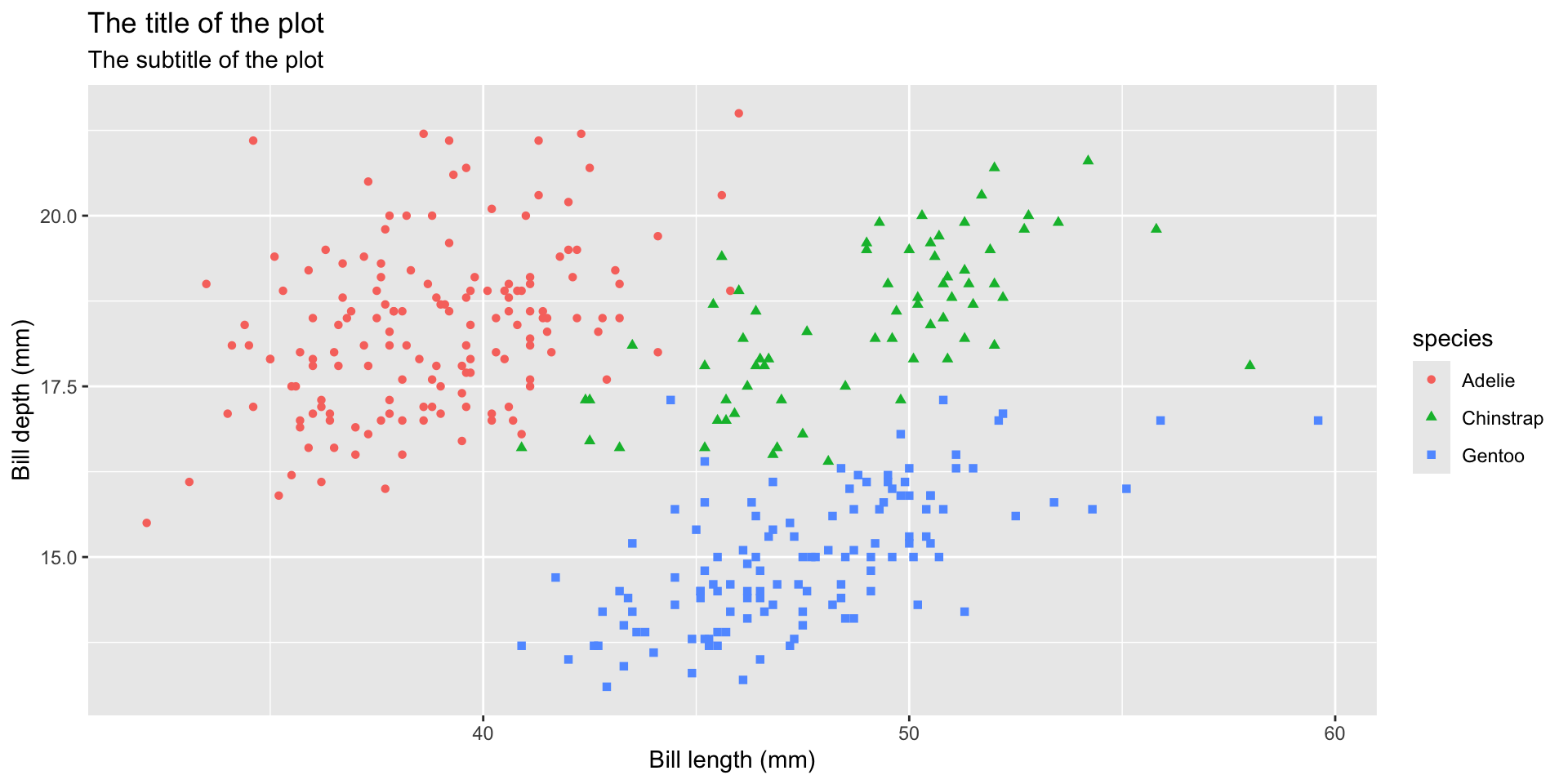
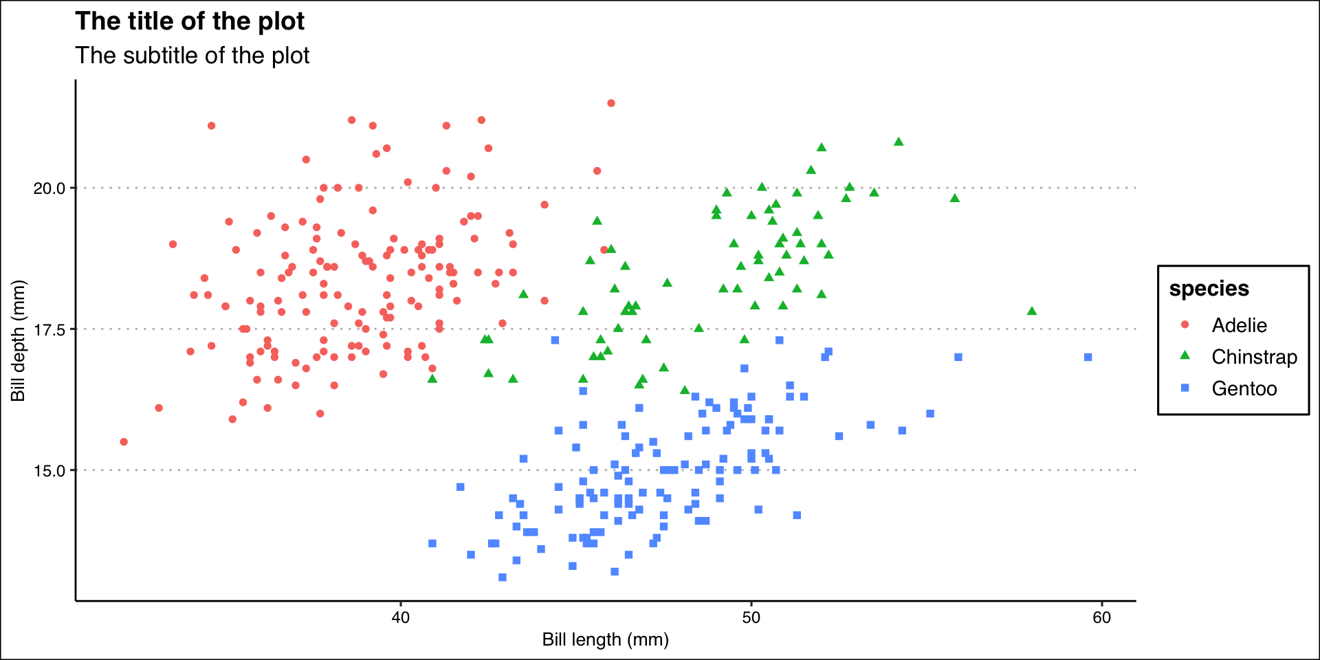
Different Shapes
Each level of the factor/category can be shown using a different shape of different color.
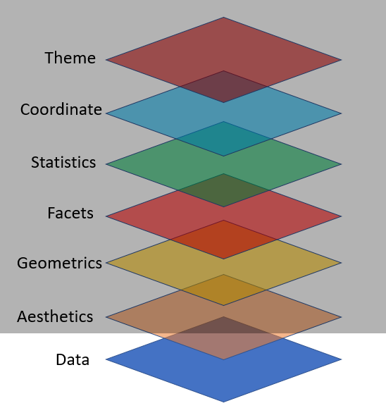
Various Themes
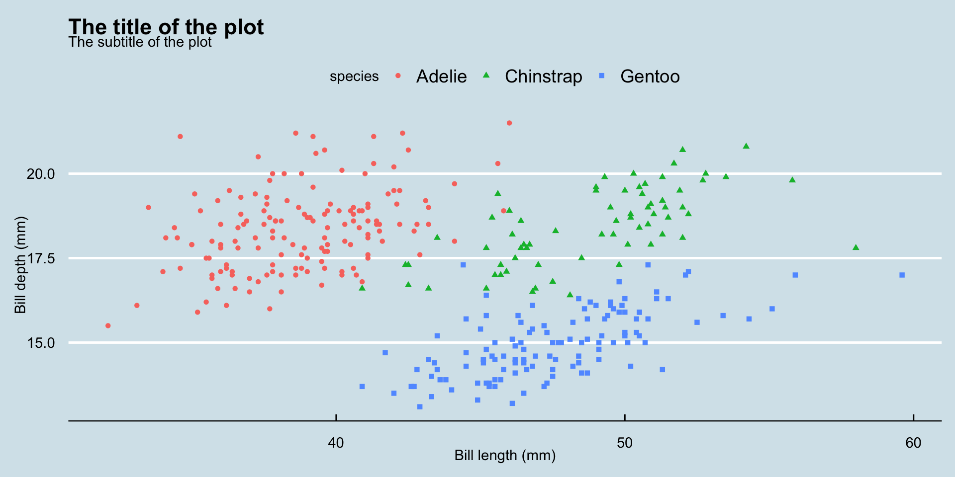
Various Themes
Various Themes
Various Themes
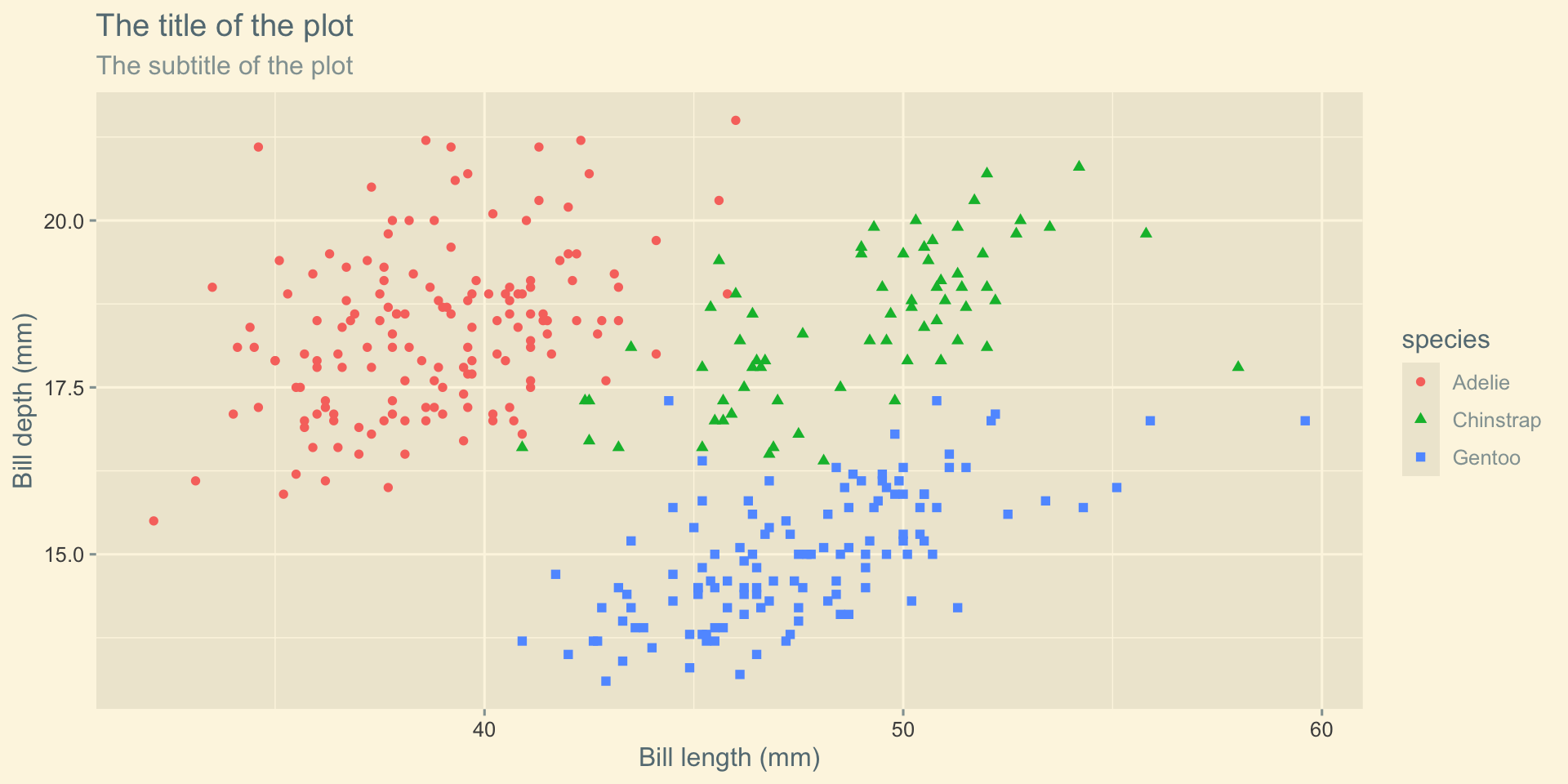
Color Palette
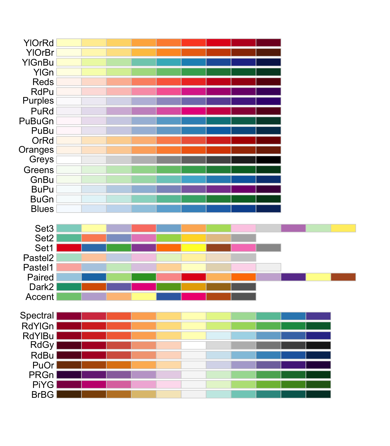
Color Palette
R package ggthemes have function to use color scheme for colorblindness. Know more
ggplot(data = penguins,
       mapping = aes(x = bill_length_mm, y = bill_depth_mm)) +
  geom_point(aes(color = species, shape = species)) +
  labs(
    title = "The title of the plot",
    subtitle = "The subtitle of the plot",
    x = "Bill length (mm)",
    y = "Bill depth (mm)"
) +
theme_clean() +
scale_color_colorblind()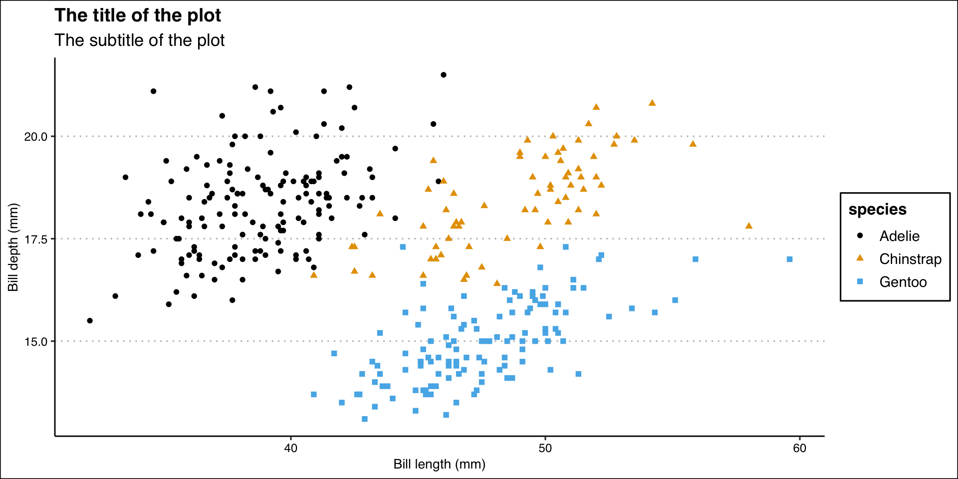
Color Palette
ggplot(data = penguins,
       mapping = aes(x = bill_length_mm, y = bill_depth_mm)) +
  geom_point(aes(color = species, shape = species)) +
  labs(
    title = "The title of the plot",
    subtitle = "The subtitle of the plot",
    x = "Bill length (mm)",
    y = "Bill depth (mm)"
  ) +
theme_clean() +
scale_color_brewer(palette = "Dark2")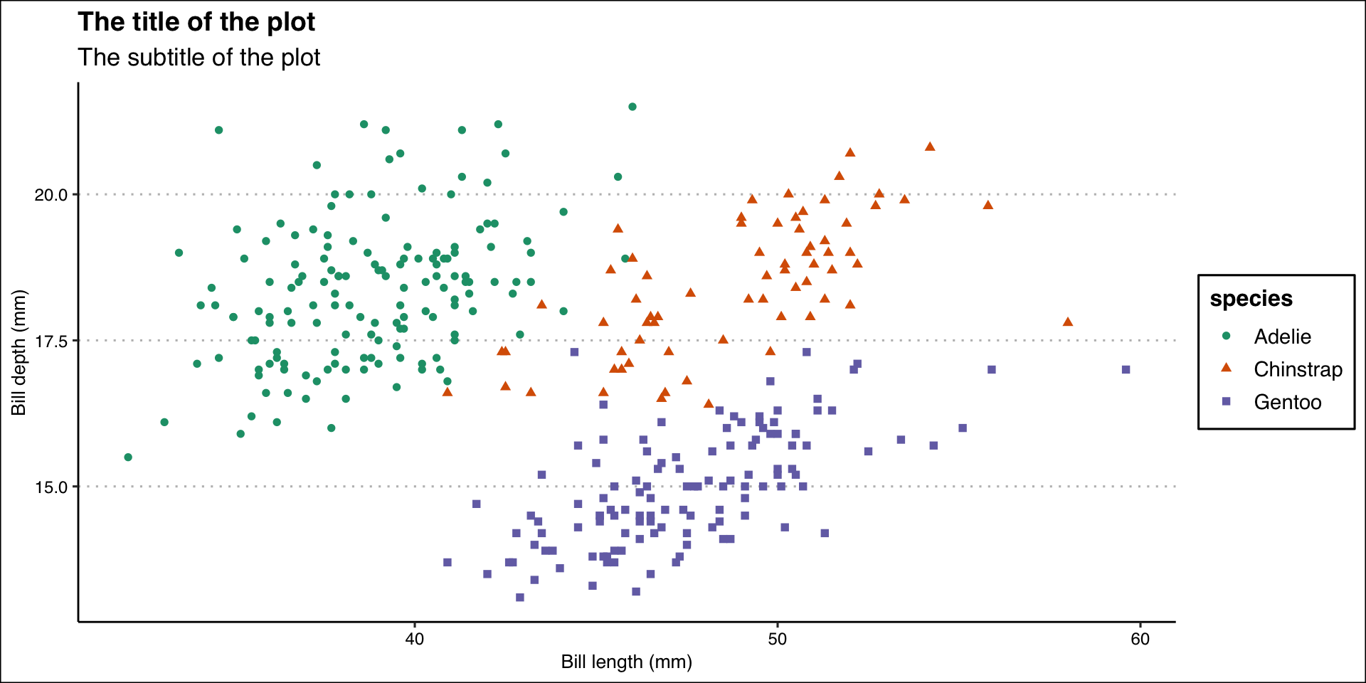
Color Palette
 [1] "BottleRocket1"     "BottleRocket2"     "Rushmore1"
 [4] "Rushmore"          "Royal1"            "Royal2"
 [7] "Zissou1"           "Zissou1Continuous" "Darjeeling1"
[10] "Darjeeling2"       "Chevalier1"        "FantasticFox1"
[13] "Moonrise1"         "Moonrise2"         "Moonrise3"
[16] "Cavalcanti1"       "GrandBudapest1"    "GrandBudapest2"
[19] "IsleofDogs1"       "IsleofDogs2"       "FrenchDispatch"
[22] "AsteroidCity1" "AsteroidCity2" "AsteroidCity3" ggplot(data = penguins,
mapping = aes(x = bill_length_mm, y = bill_depth_mm)) +
geom_point(aes(color = species, shape = species)) +
labs(
title = "The title of the plot",
subtitle = "The subtitle of the plot",
x = "Bill length (mm)",
y = "Bill depth (mm)"
) +
theme_clean() +
scale_color_manual(values = wes_palette("BottleRocket2", n = 3))
Export Plot
Export/save plot as pdf, jpg or png file.
ggplot(data = penguins,
       mapping = aes(x = bill_length_mm, y = bill_depth_mm)) +
  geom_point(aes(color = species, shape = species)) +
  labs(
    title = "The title of the plot",
    subtitle = "The subtitle of the plot",
    x = "Bill length (mm)",
    y = "Bill depth (mm)"
  ) +
  theme_clean() +
  scale_color_manual(values = wes_palette("BottleRocket2", n = 3))
ggsave("penguins-plot.pdf")